FORM

FORM: Robot Manipulation through Direct Material Law Identification

From Observed Response to Material laws

  • 1Mechanical Engineering, UC Berkeley
  • 2Electrical and Computer Engineering, UT Austin
  • 3Civil, Architectural and Environmental Engineering, UT Austin
  • 4Oden Institute, UT Austin
  • 5Aerospace Engineering and Engineering Mechanics, UT Austin

*Corresponding author: stepa@berkeley.edu

Identify material laws.
Plan robot actions.

Same action. Different materials. Different outcomes.

  1. 01
    Observe one interactionMaterial motion and contact forces
  2. 02
    Recover an explicit material lawOne linear least-squares solve on the weak form, with no differentiation through simulation
  3. 03
    Use that law to plan robot actionsNew tasks and geometries, without refitting
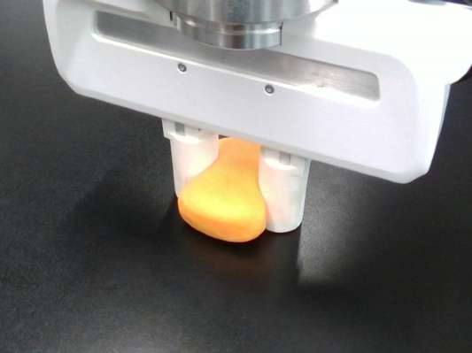
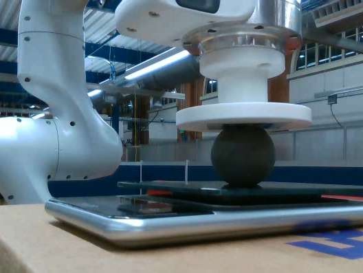
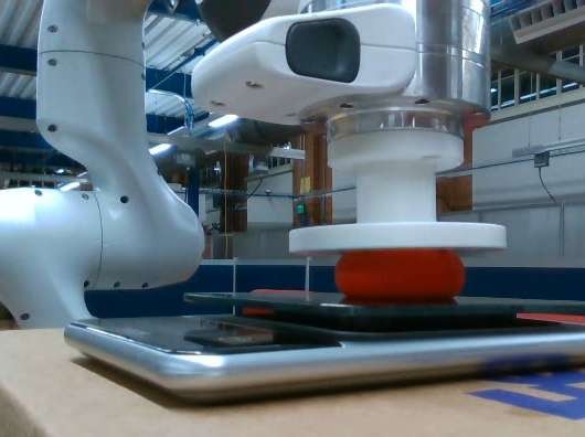
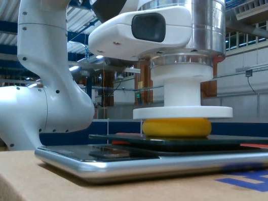
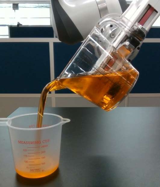
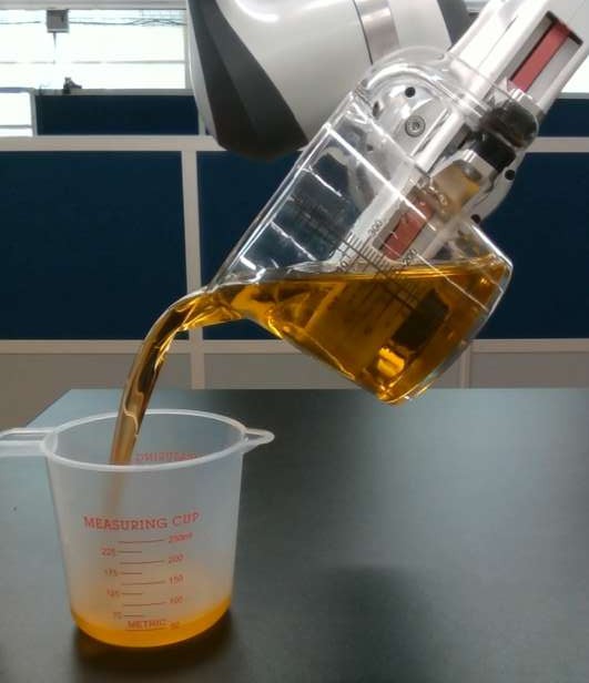
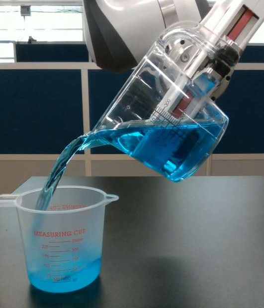
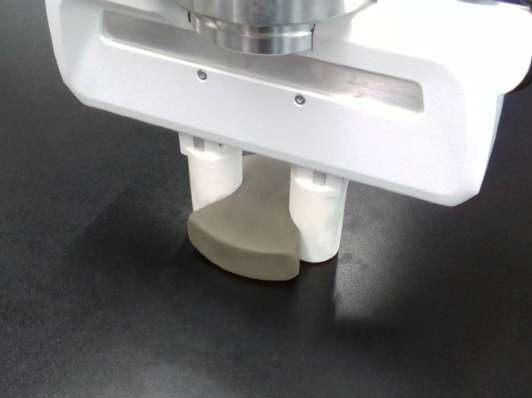
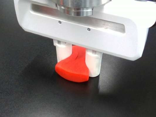
PlasticinePlay-DohButter slime Pinch to 25 mm A two-finger gripper pinching gray plasticine The same pinch on red Play-Doh The same pinch on yellow butter slime Press at 10 N A plate pressing a gray plasticine sphere The same press on a red Play-Doh sphere The same press on a yellow butter slime sphere Glycerol90% glycerolWater Pour at 10°/s The robot pouring glycerol from a tilted cup The same pour with 90% glycerol The same pour with water
From the same starting shape, the same 25 mm pinch or 10 N press deforms each material differently, and the same 10°/s pour flows differently for each liquid.

Video

FORM in three minutes

Narrated through on-screen captions; the video has no audio track.

Transcript

0:00 Overview

Different materials respond differently to the same action. We observe how the material moves during one interaction. Our method, FORM, identifies a material law. We use the identified law to plan new actions for new geometries.

0:13 Observe

First, we record the material as it deforms. With RGB-D, we reconstruct the shape assuming symmetry around the pressing axis. We keep the volume fixed, so the material spreads sideways as it flattens. We infer the flow inside from the surface motion, assuming no slip at contacts. Then we follow particles through this flow to recover their 3D paths. With stereo, we track the same texture in two views to recover surface motion. From the surface motion, we estimate how the interior moves. The motion and measured contact forces then go into material identification.

0:45 Identify and plan

Which material law explains the motion we just observed? We weight Newton’s law and integrate over space and time. Our test fields cancel the pressure term, leaving only deviatoric stress. We express stress using known responses and unknown coefficients. Linear least squares gives us the coefficients of the material law. Keeping the law fixed, we plan new robot actions in simulation. Finally, we execute that plan on the real material.

1:13 Rod insertion

From bending and force, we identify each material’s stiffness. Our task is rod insertion: a new action and geometry. Matched ID uses the rod’s identified law; swapped ID uses the other material’s law.

1:25 Golf putting

We reuse the material laws identified from bending. We plan forward-stroke duration and aim angle to stop the ball on target. Matched plans succeed; swapped plans miss.

1:35 Simulated shaping

From pressing, we identify stiffness and yield stress for each material. Keeping those laws fixed, we plan six pinches to shape a larger block into an X. Both matched plans give lower surface error.

1:50 Hardware shaping

For each material, one press identifies stiffness and yield stress. We use those laws to predict a separate, lower-force press. Next, we plan four pinches to shape fresh specimens into an X. Here, the robot executes the plan on a fresh Play-Doh specimen. The identified laws stay fixed throughout planning and execution. After rigid alignment, footprint overlap is 72 to 78 percent.

2:20 Pouring

We identify an effective viscosity from a single glycerol pour. We keep it fixed and plan the cup’s tilt for each of six target volumes. Across all six targets, the largest mean error is 3.8 milliliters. Water overpours when we use the same commands planned for glycerol.

2:46 Takeaways

FORM identifies a material law from one robot interaction. We identify material laws without backpropagation. We use the law in MPM to predict motion and plan actions. We reuse the identified material law for new actions and geometries.
Abstract

Every unfamiliar deformable material presents a robot with unknown physical properties and an unknown response to force and motion, making rapid online identification essential for reliable manipulation. We present FORM (From Observed Response to Material laws), which identifies material behavior from a single robot interaction and reuses the recovered model to plan manipulation under new actions and geometries. We convert observed material motion and contact forces into linear equations via weak-form momentum balance with material parameters as unknowns, and assemble them in the same MPM discretization used for forward prediction, reducing identification to a single least-squares solve whose solution is used directly by the simulator without refitting or conversion. Across four material classes, this reduces identification time from roughly 10–25 minutes for iterative baselines to 2–5 seconds, while retaining competitive accuracy on new motions, initial conditions, and geometries. We demonstrate the approach on elastic rod insertion, golf putting with an elastic club, elastoplastic shaping, and target-volume pouring, where models identified from one interaction are reused to plan different motions or manipulate different geometries. The method estimates elastic properties within 3.4% and elastoplastic properties within 2%, achieves 72.4–77.8% IoU in hardware shaping, and limits the largest mean pouring error to 3.8 mL over 60–160 mL targets.

Method

Recover the material law. Plan the robot action.

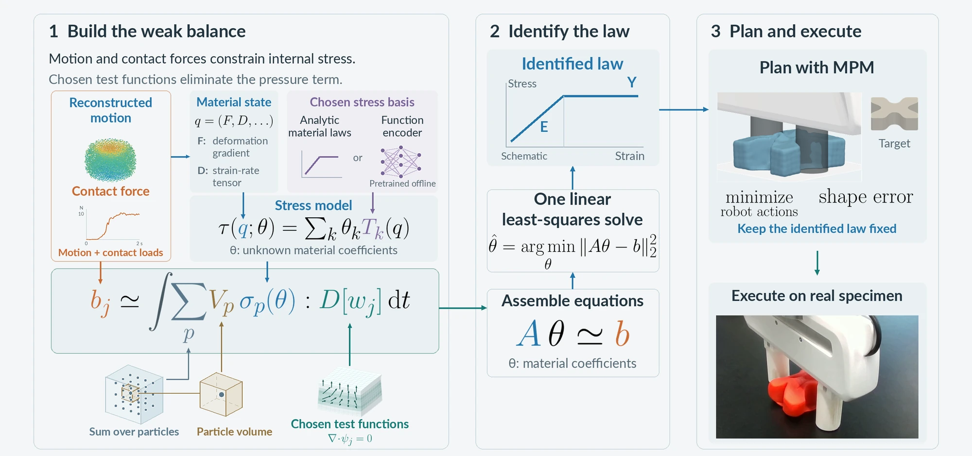
FORM holds the observed motion fixed and asks which material law explains it. Weighted momentum balance turns that question into a linear system in the material coefficients, assembled in the same MPM discretization the robot later uses to predict new actions.

Method overview in three panels. Build the weak balance: reconstructed motion and contact force, the material state, and a chosen stress basis enter an integral weighted by test functions. Identify the law: one linear least-squares solve gives stiffness E and yield stress Y. Plan and execute: MPM plans robot actions toward a target shape with the law held fixed, and the plan runs on a real specimen.
1 Tracked motion and contact force enter a weak momentum balance. 2 One least-squares solve returns the material coefficients. 3 MPM plans new actions with the identified law held fixed, and the robot executes the plan.

01Pressure drops out

Weighting momentum balance with a smooth test field ψj and integrating by parts moves derivatives from stress onto the weight. Divergence-free fields, ∇·ψj = 0, remove the unknown pressure for every pressure field and leave the deviatoric stress to identify.

Integral of tau(theta) double-dot D[psi_j], minus the integral of p times the divergence of psi_j, which is zero when psi_j is divergence-free, equals the integral of rho (g minus a) dot psi_j.

02No measured accelerations

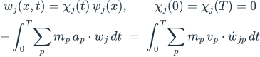
Accelerations estimated from tracked motion are imprecise at high deformation rates. Space–time weights that vanish at both ends of each window let integration by parts replace acceleration with the known rate of change of the weight along each track.

w_j(x, t) = chi_j(t) psi_j(x) with chi_j zero at both ends of the window, so minus the time integral of the sum of m_p a_p dot w_j equals the time integral of the sum of m_p v_p dot the rate of change of w_j along particle p.

03Linear in the unknowns

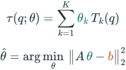
Stress is a combination of candidate responses, either analytic laws or pretrained function-encoder bases. Each may depend nonlinearly on deformation, but only linearly on the coefficients θ, so every test field adds one linear equation and one least-squares solve returns θ.

tau(q; theta) = sum over k of theta_k T_k(q); theta-hat = argmin over theta of the squared norm of A theta minus b.

04The simulator’s own basis

With the MPM quadratic B-splines as test fields, each weighted balance is the simulator’s internal-force assembly under particle quadrature. The identified coefficients go straight into MPM, without refitting or conversion.

psi_(i,d)(x) = N_i(x) e_d; the integral of sigma double-dot D[psi_(i,d)] is approximately the sum over particles of V_p e_d-transpose sigma_p grad N_i(x_p), which equals minus e_d-transpose times the MPM internal force at node i.

Plan with the identified law

With θ̂ held fixed, MPM predicts the outcome of candidate motions, and the planner searches a small set of motion parameters for the lowest task cost. Plans run open loop: measurements during execution never update the model.

u-star(theta-hat) is in the argmin over admissible motions u of the task cost J of the predicted trajectory S_theta-hat(x_0, u) and the goal G.

Results

Identify once. Plan new actions and geometries.

Every task identifies the law from a single probe and keeps it fixed. Matched ID plans with the material’s own law; swapped ID plans with the other material’s law.

2–5 sto identify a law with FORM from full observations, vs. roughly 10–25 min for iterative baselines
≤ 3.4%error in identified elastic moduli; under 2% for elastoplastic parameters
72–78%footprint IoU after open-loop shaping of three real materials
3.8 mLlargest mean pouring error over six targets from 60 to 160 mL

Elastic rod insertion and golf putting

Simulation

A bending probe identifies Young’s modulus from tracked surface texture and pusher force: 80.61 kPa for material A (true 80 kPa) and 248.11 kPa for B (true 240 kPa). The same laws then plan two tasks with new actions and geometry.

Rod insertion. Choose gripper height and tilt to thread an 8 mm rod through a 12 mm hole.
  • Matched: both rods insert without wall contact; RMS tip error 0.355 mm (A) and 1.042 mm (B)
  • Swapped: both rods hit the wall
Golf putting with an elastic club. Choose forward-stroke duration and aim angle to stop the ball in a 35 mm-radius target 612 mm away.
  • Matched: 2.36 mm (A) and 19.06 mm (B) from the target center
  • Swapped: 350.47 mm and 158.67 mm; both miss

Elastoplastic shaping

Simulation

Materials A and B share their stiffness, but B’s yield threshold is ten times higher. A flat-plate press on a 30 × 30 × 25 mm specimen identifies both parameters, and six planned pinches then shape a larger block into an X.

Rows are materials; columns are whose identified law planned the pinches.

Identified from one press

MaterialE (kPa)Y (kPa)
A80.795 / 801.015 / 1
B81.396 / 8010.184 / 10

Identified / true values; every error is below 2%. Hencky elasticity with von Mises plasticity.

Surface error after six pinches

PlanAB
Matched ID0.883 mm1.256 mm
Swapped ID1.226 mm1.739 mm

Mean closest-point distance to the target surface, 1 s after the fingers withdraw.

Identification press, a planned pinch, the X-shaped target, and final shapes for matched and swapped plans of materials A and B, with dashed target outlines
Identification press, a planned pinch, and the target, followed by final shapes for matched and swapped plans. Dashed outlines mark the target.

Pressing and shaping real materials

Hardware

One press of a 45 mm sphere, reconstructed from two RealSense D435 cameras under constant volume, identifies stiffness and yield stress for red Play-Doh, yellow butter slime, and gray plasticine. With those laws fixed, MPM predicts a separate press, and the planner chooses four pinches that shape fresh 60 × 60 × 25 mm blocks into an X, executed open loop.

A separate, lower-force press (top) and the force-driven MPM prediction from the identified laws at matching times (bottom).
Four planned pinches, executed open loop on a fresh Play-Doh block.
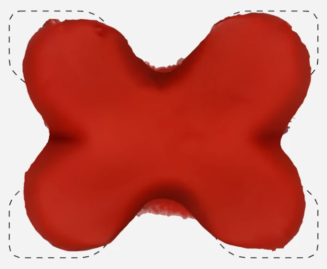
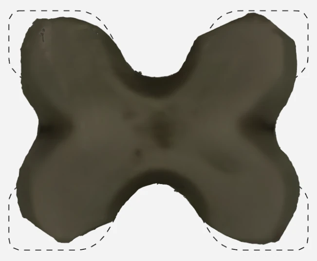
Scan of the shaped Play-Doh X inside the dashed target outlinePlay-Doh75.7%
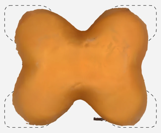
Scan of the shaped butter slime X inside the dashed target outlineButter slime72.4%
Scan of the shaped plasticine X inside the dashed target outlinePlasticine77.8%
Scans after four pinches, rigidly aligned to the dashed target without scaling. Numbers are footprint IoU.

Pouring a target volume

Hardware

A single 60° exploratory pour of glycerol gives an effective Newtonian viscosity of 3.44 Pa·s from a reduced weak-form balance at the spout, using the receiver volume tracked on video and the cup motion from the robot’s joint trajectory. With that viscosity and an effective wall-contact coefficient (calibrated in MPM from the same pour) held fixed, MPM selects the final tilt angle for six targets from 60 to 160 mL. The commands are frozen before five hardware repeats per target.

The 60° identification pour on hardware and its MPM replay.
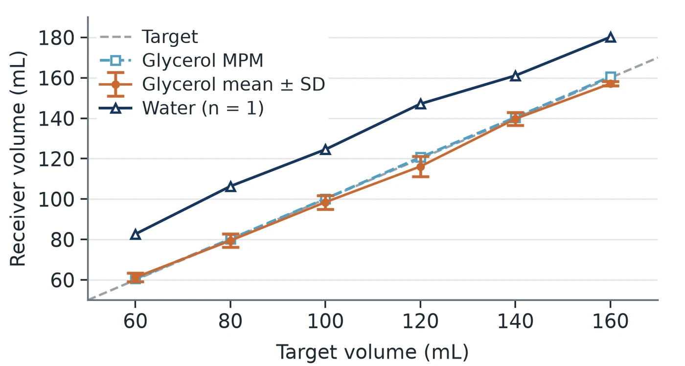
Receiver volume versus target volume: glycerol hardware means and MPM predictions follow the target line from 60 to 160 mL, while water poured with the same commands lies above it at every target
Glycerol: frozen MPM predictions and hardware mean ± SD over five trials per target. Water: one trial per target, poured with the commands planned for glycerol.
Six receiver cups labeled target to measured volume: 60 to 59, 80 to 84, 100 to 101, 120 to 123, 140 to 137, and 160 to 157 mL
Repeat 2: target → measured receiver volume (mL). Across all six targets, the largest mean error is 3.8 mL; water overshoots every target.

Benchmark

Seconds instead of minutes

Identification accuracy and solve time on the NCLaw dataset and setup: four materials, one trajectory each. Mean loss is averaged over three generalization tests: extended time, unseen initial conditions, and a new geometry.

Method Jell-O Sand Plasticine Water
Mean lossTime (s) Mean lossTime (s) Mean lossTime (s) Mean lossTime (s)
NCLawNeural constitutive law 5.2×10−41513.2 1.6×10−41305.6 1.2×10−41300.2 5.7×10−41306.8
Diff. Sys-IdOracle: exact law given 1.2×10−8715.8 6.3×10−131132.8 1.6×10−101028.4 4.0×10−9556.2
FORM (Fn Enc.)Pretrained bases by material type 3.5×10−45.2 3.3×10−80.1 2.9×10−65.3 2.3×10−64.8
FORM (Full)Full information 5.1×10−64.4 1.4×10−82.4 5.2×10−74.7 2.3×10−62.2
FORM (No stress)Observations without stress 5.1×10−63.5 2.0×10−86.0 5.2×10−76.5 2.3×10−61.6
FORM (Pos. only)Positions only 1.3×10−53.5 1.0×10−512.8 4.6×10−621.8 1.0×10−24.6
  • Diff. Sys-Id is an oracle: it differentiates through MPM trajectories with the exact constitutive law given.
  • Full uses full information, including stress; No stress drops the stress observations; Pos. only uses positions alone. For plasticine and sand, positions do not determine the elastic state, so Pos. only scans forward rollouts over the plastic parameter with the elastic moduli fixed at their true values.
  • Fn Enc. uses pretrained function-encoder bases selected by material type, for when the exact law is unknown.
  • Bold marks the lowest-loss non-oracle result for each material and its solve time.

Code

Code and reproduction

The repository contains the weak-form identification, a GPU MPM solver in NVIDIA Warp with the added constitutive models, the pipelines for rod insertion, golf putting, shaping, and pouring, a reproduction runner that recomputes the paper’s material estimates and checks saved results, and the renderer for the video and slides.

Recordings and saved simulation data will be released separately.

The MPM solver builds on warp-mpm by Zong et al.; see AUTHORS.md for attribution.

Setup · Linux, Python 3.12
git clone https://github.com/form-robots/FORM.git
cd FORM
uv venv --python 3.12
uv pip install --python .venv/bin/python -r requirements-lock.txt
uv pip install --python .venv/bin/python --no-deps -e '.[paper,dev]'
source .venv/bin/activate

Citation

BibTeX

BibTeX
@misc{tretiakov2026form,
  title  = {{FORM}: Robot Manipulation through Direct Material Law Identification},
  author = {Tretiakov, Stepan and Zhao, Ruihan and Hsiao, Cheng-Hsi and Li, Xingjian and
            Thorpe, Adam and Iqbal, Hassan and Chinchali, Sandeep and Topcu, Ufuk and Kumar, Krishna},
  year   = {2026},
  url    = {https://form-robots.github.io/}
}